The Cross-Section Expected Stock Returns

Contents

1. Abstract & Introduction

2. Preliminaries

3. β estimates

4. The relation between Average return and beta , Average return and size(ME)

5. The relation between Average return and E/P , Leverage , BE/ME

6. A Parsimonious Model for Average returns

7. Conclusion

   1. Abstract & Introduction

Two easily measured variables, size and book-to-market equity, combine to capture the cross-sectional variation in average stock returns associated with market beta, size, leverage, book-to-market equity, and earnings-price ratios. Moreover, when the tests allow for variation in beta that is unrelated to size, the relation between market and average return is flat, even when Beta is the only explanatory variable.

There are several empirical contradictions of the SLB Model

1. size effect of Banz(1981)
   • ME is the explanation of the cross-section of average returns provided by market beta.
2. positive relation between leverage and average return of Bhandari (1988)
   • leverage helps explain the cross-section of average stock returns in tests that include size as well as beta
3. positive relation between BE/ME and average return of Stattman and Rosenberg, Reid and Lanstein (1985)
4. E/P help explain the cross-section of average returns of Basu (1983) and E/P is a catch-all proxy for unnamed factors in R of Ball(1978)
5. relation between beta and average return disappears during the more recent 1963-1990 of Reinganum(1981) and Lakonishok and Shapiro(1986)

• ME , BE/ME , Leverage , E/P are scaled versions of price.

• it is reasonable to expect that some of them are redundant of Keim(1988)

  2. Preliminaries

논문의 1장은 예비 절차(Preliminaries)로 분석에 있어서 사용되는 데이터와 시장 베타의 측정 기준이 정리되어 있다.

1. Fama-French 3 factor model 의 데이터 관측 시기는 1963-1990년 간이다.

2. 데이터 분석은 비금융회사만을 포함하고 있다.(Data analysis includes only non-financial companies.)

   • why ? :
     • 비금융회사에서 높은 레버레지는 재정적으로 불안정하다는 것을 의미하지만, 금융회사의 경우 정상적인 경우일 수 있다.
     • A high leverage in a non-financial company means financially unstable, but it may be normal for a financial company.

3. 회계 변수들은 그것이 설명하는 수익률보다 먼저 확인 가능하다.(Accounting variables can be checked before profit rate which it explains.)

   • So what did they do :
     • t-1 년 (1962-1989) 에 있는 모든 회계연도 말의 회계 자료를, t 년 7월부터 t+1 년 6월까지의 수익률과 대응시킨다.
     • 회계년도 말과 수익률 테스트 간에 최소 6개월의 차이를 둔다.

     • The six month gap between financial reporting and realized returns insure the reflection of all information into the stock pricing

     • WHICH data they used and WHEN did they take them :

     • BE/ME , LEVERAGE , E/P , A : t-1년의 12월 말 시가총액(ME)을 사용

     • ME : t 년의 6월 시가총액을 사용

     • pre-ranking beta : 24 to 60 monthly returns(as available) in the 5 years before July of year t. (Only using NYSE)

     • pre-ranking beta , post-ranking beta 를 계산할 때는, 전월 수익률과 당월 수익률을 합한 합산 베타를 적용한다.

        - return_p,t = beta_0 + `beta_1` * r_m,t_1 + `beta_2` * r_m,t + resid_p
        - beta_p = beta_1 + beta_2

3. β estimates

• 각각의 베타들을 추정하기 위해서는, 회귀분석 작업이 필요하다. 즉, 모든 베타들에 대해서 회귀 분석 작업이 들어간다.
  • 베타 : ME , E/P , A/ME , A/BE , β_m , BE/ME
  • 주식별 베타 수치는 별도의 프로세스을 추가적으로 적용하여 만들어진다.
  • 포트폴리오 접근법 사용 why? :
    • 사이즈 효과를 베타로부터 제거하기 위해서 , to allow for variation in beta that is unrelated to size.

Calculating Post - ranking beta

1. NYSE 주식을 시가총액 순으로 10분위 기준점을 잡는다. (10*1)
   • NASDAQ이 표본에 추가되면, 포함된 시점부터 대부분의 포트폴리오에 small_cap 만 포함된다.
2. 사이즈 포트폴리오 내에서, NYSE 주식을 pre-ranking beta 순으로 정렬해(subdivide) 10분위 기준점을 잡는다. (10*10)
   • 사이즈-베타 포트폴리오는 7월~6월동안의 데이터로 만들어지고, 6월말에 리밸런싱된다.
3. 베타를 측정하는 방법 :
   • 동일 가중 월별 수익률을 만든 size-beta portfolio에 대해서 12달 계산한다.(7~12)
   • 1년마다 포트폴리오를 리밸런싱하고 같은 프로세스 아래에서 1963~1990 으로 총 330달에 대한 수익률을 계산한다.
   • NYSE , AMEX , NASDAQ 의 value-weighted 포트폴리오의 수익률을 시장 수익률의 대용치로써 사용해 베타를 측정한다.

full-time beta estimates

• After assigning firms to the size-beta portfolios in June, we Calculate the equal-weighted monthly returns on the portfolios for the next 12 months, from July to June.
• In the end, we have post-ranking monthly returns for July 1963 to December 1990 on 100 portfolios formed on size and pre-ranking betas.
• Then FF estimates betas using the full sample (330 months) of post-ranking returns on each of the 100 portfolios, with the CRSP value-weighted portfolios of NYSE , AMEX , and NASDAQ used as the proxy for the market. (FF did test with equal-weighted portfolio as proxy of the market. The result was similar with before.)

Stocks Sorted on ME then Pre-Ranking beta

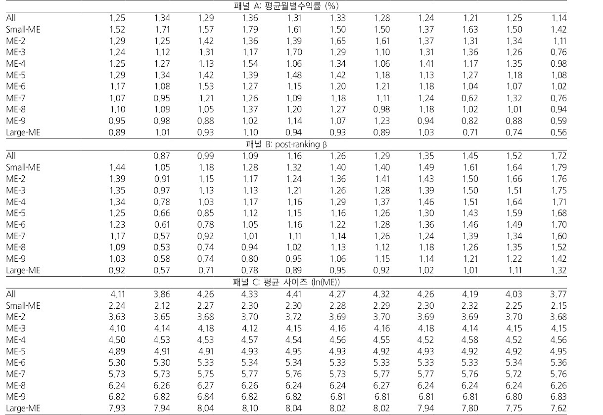
위의 표를 보고 베타에 대해 알 수 있는 2 가지 사실

• 각 사이즈 분위 안에서 post-ranking 베타는 pre-ranking 베타의 순서를 매우 유사하게 재현한다.
  • pre-ranking 베타가 실제 post-ranking 베타를 유사하게 재현한다. (재현력 , 예측력)
• 베타의 순서는 변형된 사이즈 순서가 아니다. -모든 사이즈 분위 내에서 ,ln(ME) 의 평균값은 베타로 정렬된 세부 포트폴리오들 간에 유사한 값을 지닌다. ——————————————————————–

  4. 평균수익률과 베타, 평균수익률과 사이즈의 관계

  • (Banz(1981))에 의하면, 사이즈와 R 은 Negative , 베타와 R은 Positive 한 상관성이 있다고 했다.

• model’s central prediction : average return is positively related to beta, The betas of size portfolios are however, almost perfectly correlated with size.
• 위의 말은, SLB에서 진행한, 베타와 수익률간의 테스트가 사이즈 효과에 의해서 왜곡되었다고 주장하는 것.

Properties of Portfolios Formed on Size or Pre-Ranking betas

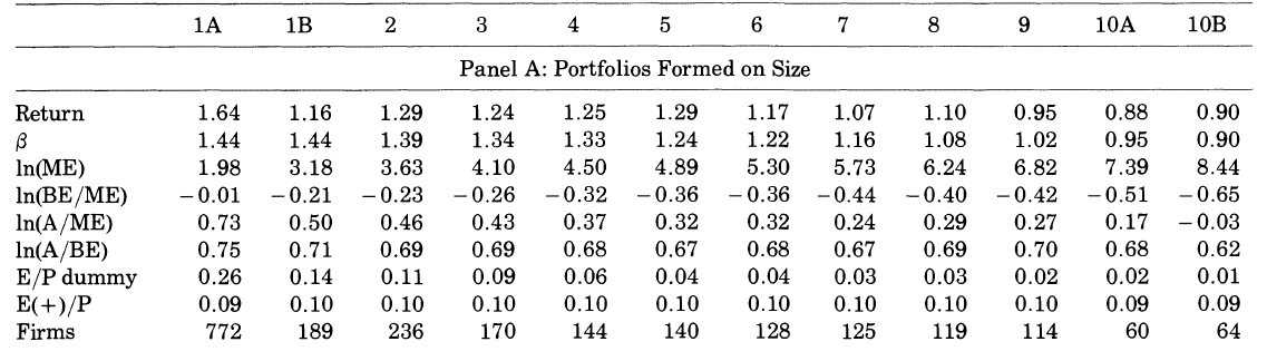
표를 보게 되면, 평균수익률과 사이즈는 역상관성, 베타는 상관성을 띄는 것으로 보인다. 즉, 사이즈 포트폴리오는 SLB 모델을 지지한다.

• 사이즈 포트폴리오 내에서 사이즈와 베타 간의 상관 관계에 의한 왜곡된 결과이다.

• beta 로 배열된 포트폴리오는 SLB 모델을 지지하지 않는다. 슈익률에 대한 스프레드가 거의 보이지 않는다.

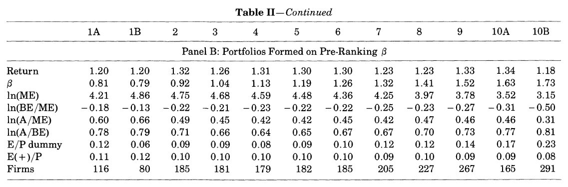
• Panel B : Portfolios Formed on Pre-Ranking β
  • β 의 10분위 수가 1A(최소극단치)일때와 10B(최대극단치)일 때의 차이가 미비하다.

  • 1969년 이후로 시장 베타와 수익률의 관계가 사라졌다!! (Reinganum(1981), Lakonishok-Shapario(1986))

  • Table I 에서 사이즈 분위 내의 post-ranking 베타의 변화에 따른 평균 수익률의 변화를 보자!

사이즈와 연동된 베타는 평균수익률과 연관이 있다. 하지만, 무관한 베타는 상관관계가 없다.

• 사이즈 <-> 베타 (Negative) , 사이즈 <-> 평균수익률(Negative) , 베타 <-> 평균수익률(Positive)

  5. Fama-Macbeth Cross_sectional Regression

• time-series averages of the slopes from the month-by-month Fama-MacBeth regressions of the cross-section of stock returns on input variables.

Average Slopes from Month-by-Month Regressions of Stock Return on betas

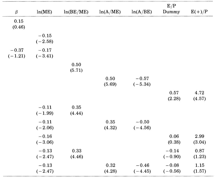
Can beta Be Saved?

• other explanatory variables are correlated with true betas
  • beta has no power when used alone to explain average Return.
• the relation is obscured by noise in the beta estimates.
  • standard error is 0.05 or less. not seems to be imprecise.

  • post-ranking beta for the portfolios almost perfectly reproduce ordering of the pre-ranking betas. (post-ranking betas are informative about the ordering)

    ~~~

• 평균 수익률(R)과 사이즈(ME) 간에는 강한 상관관계가 있다.
• 평균 수익률(R)과 베타(β) 간에는 상관성이 없다. ~~~ ——————————————————————–

  6. 평균수익률과 E/P , Leverage , BE/ME의 관계

  본 장에서는 BE/ME가 Return 과 강한 상관관계가 있음을 알아본다. (심지어 사이즈 효과보다 더 크다.)

average returns for July 1963 to December 1990 for portfolios formed on ranked values of BE/ME or E/P.(one-dimensional yearly sorts)

Properties of Portfolios Formed on BE/ME and E/P

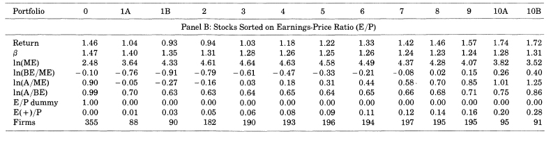
• 평균수익률(R)과 E/P 의 관계는 U자형이다.
• 평균수익률(R)과 BE/ME 의 관계는 정상관성을 띈다. 스프레드의 크기가 사이즈 포트폴리오의 2배에 달한다.
  • 음수 BE/ME는 제외하였다.(50개 기업에 불과하고 특정 기간에 집중되어 있다.)
• Interpretation of BE/ME :
  • BE/ME에서 장부가치는 잘 변하지 않는다. 이에 따라 고 BE/ME는 낮은 ME를 의미한다. 즉, 낮은 시장가치를 의미하는 것이다. 즉, 높은 BE/ME 는 기업의 부정적인 전망 신호를 의미한다.

• 베타(β)와 BE/ME 의 관계는 상관성은 보이지 않는다.

  ~~~

• BE / ME 가 사이즈와는 다른(distinctive) 중요한 설명변수이다.
• BE / ME 가 레버리지 변수의 역할을 대체하고 , E / P 의 역할을 대체한다. ~~~ ——————————————————————–

1. BE / ME :
   • BE / ME 와 ME 가 Cross_sectional Regression 시에 대체되지 않고, 두 베타 모두 유의미하다.
2. Leverage :
   • 장부 레버리지(A/BE) , 시장 레버리지 (A/ME) 두 가지 변수 사용.

   • 로그함수가 평균수익률에서 레버리지 효과 포착이 용이하다.즉, ln(A/BE) , ln(A/ME) 을 사용한다.

   • 장부 레버리지는 Negative , 시장 레버리지는 Positive

   • 장부 레버리지와 시장 레버리지의 절대값은 유사하다.

   • (시장 레버리지) - (장부 레버리지) 변수가 유의미해진다. ln(A/ME) - ln(A/BE) = ln(BE/ME) 가 된다. 즉, BE/ME 와 leverage는 강한 연관성이 존재한다.

   • StoryLine :
     • BE/ME 가 높을 경우는,
       1. low ME -> Negative prospect
       2. high BE -> Implicitly leveraged(impose by Market)
3. E / P :
   • 기대수익률(R) 에서 누락된 위험 요인들을 포괄하는 변수라고 규정한다.(Ball(1978))
   • BUT
   • 사이즈를 더하면 더미변수의 영향력이 사라진다.
   • 사이즈와 BE/ME를 함께 하면, 더미변수와 E/P 변수의 영향력이 흡수된다.

Average Monthly Returns on Portfolios Formed on Size and BE/ME

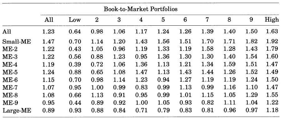
• 사이즈를 통제하면 BM/ME 가 평균 수익률의 강한 변동을 포착하게 되고,BM/ME 를 통제하면, 수익률에 사이즈 효과가 남는다.

1. 사이즈와 관련 없는 베타는 평균 수익률과의 연관성이 존재하지 않는다.

2. 평균 수익률에 있어 시장 레버리지(A/ME)와 장부 레버리지(A/BE) 간의 반대되는 역할은, BE/ME에 의해 포착된다.

3. E/P와 평균 수익률 간의 반상관성은(Negative) BM/ME 에 의해 흡수된다.

Parsimonious Model for Average returns

• 사이즈를 통제한 베타는 평균 수익률과의 신뢰성있는(reliable) 상관관계가 없다.

• 평균 수익률에 대한 시장 레버레지와 장부 레버레지의 반대적 역할은 BE/ME에 의해서 포착된다.

• E/P와 평균 수익률 간의 관계는 사이즈와 BE/ME에 의해서 흡수된다.

A. Average Returns , Size and BE/ME

• 사이즈를 통제한 BE/ME 는 평균 수익률에 대한 강한 변동성을 보인다.(not-flat)
• BE/ME를 통제한 사이즈도 평균 수익률과 negative relation을 보인다.

B. The interaction between Size and BE/ME

• 사이즈와 BE/ME는 반상관성을 띈다.(-0.26)

  시가총액이 낮은 즉, 사이즈가 작은 기업은 좋지 않은 전망을 가질 확률이 높아지고, 낮은 주가와 높은 BE/ME를 가지는 경향을 가진다.(be likely to)
  

• 반상관성을 띄지만, 각 변수들을 통제했을 때, 상대 변수가 큰 변동성(substantial variation)을 보여주기 때문에, 이러한 상관성을 과대해석되면 안된다.

C. Subperiod Averages of the FM slopes

Subperiod Average Monthly Returns on the NYSE Equal-Weignted and Value-weighted portfolios and Subperiod means of the intercepts and slops from the Monthly FM cross-sectional regressions of Returns

• in FM regressions, the intercepts means :
  • explanatory variable = 0
• in FF tests, the intercepts means :
  • small stocks (ln(me)=0, me = 1 million)
  • high BE/ME (ln(BE/ME) = 0 , BE/ME = 1)
• 베타는 여전히 중요한 요소가 아닌 것으로 보인다.
• 사이즈는 마지막 168개월에서 약해지지만, 해당 기간에 대한추론(inference)이 즉, t(Mn)이 약해진다.
• BE/ME는 여전히 가장 강력한 요소로 작용한다.
  • subperiod 의 slope 평균이 전체 slope과 유사하다.(0.35)

D. Beta and the Market Factor : Caveats

• Meaning of Caveats :
  • a warning to consider something before taking any more action, or a statement that limits a more general statement

• The average premiums(slope) for beta , size , BE/ME depend on the definitions of the variables used in the regressions.

• Redefinition of explanatory variables can produce different regression slopes and perhaps different inferences about average premiums, including possible resuscitation of a role of beta.

• the tests here are restricted to stocks. It is possible that including other assets will change the inferences about the average premiums.

• But, FF argued different approaches to the tests are not likely to revive the SLB model.

• Stambaugh’s(1982) evidence that tests of the SLB model don’t seem to be sensitive to the choice of a market proxy.

• Therefore, FF said that it is likely to be found in a multi-factor model that transforms the flat simple relation between R and beta into a positively sloped conditional relation.

Conclusions and Implications

1. 평균 주가수익률이 시장 베타와 정상관성이 있다는 SLB 모델의 중심 예측을 지지하지 않는다.
2. 사이즈, E/P , 레버레지 , BE/ME 같은 변수들은 기업의 주가를 변형한 변수들로, 회귀분석 과정에서 평균수익률을 설명함에 있어, 몇몇 변수들은 불필요하다고(redundant) 할 수 있다.
3. 1963~1990 년 기간에 대해, 사이즈와 BE/ME 변수가 나머지 모든 변수들과 연관된 평균주가수익률의 횡단면 변화를 포착한다.

A. Rational Asset-Pricing Stories

- FM regressions always impose a linear factor structure on returns and expected returns that is consistent with the multi-factor asset-pricing models of Merton and Ross.

- test impose a rational asset-pricing framework on the relation between R and ME and BE/ME.

- FF inquires the economic explanation for the roles for explanatory variables.

• Chan , Chen and Hsieh(1985) argue that the relation between size and R proxies for a more fundamental relation between R and economic risk factors.
  • size effect is the difference between the monthly returns on low-grade and high-grade corporate bonds, which in principle captures a kind of default risk in returns that is priced.

• Chan , Chen (1991) argue that the relation between size and R is a relative- prospects effect. relative-prospects effect results in a distress factor in R that is priced in expected R.

• If, the market is rational, the BE/ME should be direct indicator.

B. Irrational Asset-Pricing Stories

• FF argued that asset-pricing effects captured by size and BE/ME are rational.

• there is strong alternative. The cross-section of BE/ME might result from market overreaction to the relative prospects of firms.

• Simple tests do not confirm that the size and BE/ME effects in average returns are due to market overreaction, at least of the type posited by DeBondt and Thaler(1985).

• One overreaction measure used by DEBondt and Thaler is a stock's most recent 3-year returns. (Their overreaction story predicts that 3-year losers have strong post-ranking returns relative to 3-year winners.) - shows no power even when used alone to explain average returns.

C. Application

• a) wheter it will persist, and b) whether it results from rational or irrational asset-pricing.

• FF said that if their results are more than chance, they have practical implications for portfolio formation and performance evaluation by investors whose primary concern is long-term average returns.

• if asset-pricing is rational:
  • ME , BE/ME must be proxy for risk. (can be used for managing and evaluating portfolios.)
• if asset-pricing is irrational:
  • might still be used to evaluate portfolio performance and measure the E(R).
  • But, the likely persistence of the results is more suspect.